

Excel Pivot Tables Tutorial: Build, Group, Slice and Refresh
Excel pivot tables tutorial with a sales example: create a pivot, use Rows, Columns, Values and Filters, show percentages, group dates, add slicers and refresh.
At Narmada Traders, the Monday meeting always starts with the same questions. Which area sold most last week? Which category is growing? Who are the top five retailers? The accountant used to answer each with a fresh set of SUMIFS formulas, and every new question meant another half hour.
Then she dragged "Area" into one box and "Amount" into another, and a summary appeared. She dragged "Category" across the top, and it became a grid.
The invoice list is the source data. The boxes she dragged into are the pivot table field areas. The grid that appeared is the pivot table, and changing the question by moving fields is pivoting.
An Excel pivot table is an interactive summary table that groups, totals, counts or averages the rows of a source table based on fields you place in its Rows, Columns, Values and Filters areas.
This tutorial uses the ten-invoice Sales Table from the formulas and functions tutorial, cleaned with the steps in data cleaning in Excel. Clean data matters more for pivots than anywhere else, because every spelling variant becomes its own row.
How do you create a pivot table in Excel?
- Click any cell inside the
SalesTable. - Go to Insert > PivotTable. Excel suggests the Table name as the range.
- Choose New Worksheet and click OK. An empty pivot and the PivotTable Fields pane appear.
- Tick or drag Area into Rows.
- Drag Amount into Values. Excel shows Sum of Amount.
That complete pivot table answers "sales by area" without a formula.
| Row Labels | Sum of Amount |
|---|---|
| Bhawarkuan | 7960 |
| Palasia | 11100 |
| Rajwada | 11640 |
| Sudama Nagar | 3480 |
| Vijay Nagar | 12860 |
| Grand Total | 47040 |
Always build pivots on an Excel Table (Ctrl+T), not a fixed range, so new invoices are picked up on refresh.
What are the four areas of a pivot table?
| Area | What it does | Narmada Traders example |
|---|---|---|
| Rows | One row in the result per unique value | Area, Retailer, Product |
| Columns | One column per unique value | Category |
| Values | The number that gets summarised | Sum of Amount, Sum of Qty |
| Filters | Limits the whole pivot to chosen items | Product = Atta 10kg |
Drag Category into Columns and the summary becomes a cross-tab:
| Sum of Amount | Beverages | Oil | Staples | Grand Total |
|---|---|---|---|---|
| Bhawarkuan | 7960 | 7960 | ||
| Palasia | 11100 | 11100 | ||
| Rajwada | 4680 | 6960 | 11640 | |
| Sudama Nagar | 3480 | 3480 | ||
| Vijay Nagar | 2600 | 5220 | 5040 | 12860 |
| Grand Total | 7280 | 15660 | 24100 | 47040 |
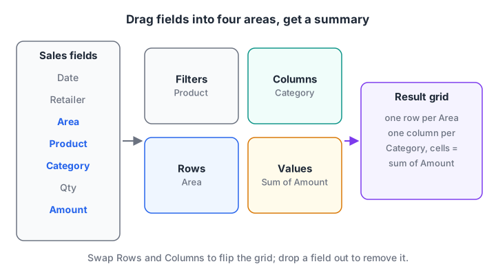
Each field you drag decides one direction of the summary. Swapping Area and Category flips the grid in a second.
Blank cells mean there were no sales for that pair. To show zeros instead, right-click the pivot, open PivotTable Options, and set For empty cells show to 0.
Quick check
Which pivot area should hold Category to show one column per category?
Fields in Columns create one column for each unique value. Rows creates one row per value, and Filters limits the whole pivot.
Changing how values are summarised
Sum, Count, Average and more
Numbers default to Sum. Text fields placed in Values default to Count. To change it, click the field in the Values area, choose Value Field Settings, and pick Count, Average, Max or Min.
Put Amount in Values twice, set the second one to Count, and you get sales and number of invoices side by side. Vijay Nagar shows ₹12,860 from 3 invoices.
Show Values As percentages
In Value Field Settings, the Show Values As tab changes what the number means without changing the data. % of Grand Total shows each area's share:
| Area | % of Grand Total |
|---|---|
| Vijay Nagar | 27.3% |
| Rajwada | 24.7% |
| Palasia | 23.6% |
| Bhawarkuan | 16.9% |
| Sudama Nagar | 7.4% |
Other useful options are % of Row Total (each category's share within an area), Difference From (change versus a previous month) and Rank Largest to Smallest.
Sort and filter inside the pivot
Right-click any value and choose Sort > Sort Largest to Smallest to rank areas by sales, as in the table above. For a top-five list, open the Row Labels dropdown and choose Value Filters > Top 10, then change 10 to 5.
How do you group dates in a pivot table?
Put Date in Rows. In current Microsoft 365, Excel often groups dates into Years, Quarters and Months automatically. If it does not, right-click any date and choose Group, then select the levels you want, such as Months and Years.
With the five April days in the sample, grouping by day gives:
| Date | Sum of Amount |
|---|---|
| 01-Apr | 9840 |
| 02-Apr | 9560 |
| 03-Apr | 10900 |
| 04-Apr | 8160 |
| 05-Apr | 8580 |
Grouping works only when every cell in the Date column is a real date. One text date such as "15.04.2026" makes Group fail. The text and date functions tutorial shows how to convert them.
Calendar quarters start in January. For India's April to March financial year, add a helper column in the source, such as =YEAR([@Date])+(MONTH([@Date])>=4), and put that in Rows instead.
Slicers, timelines and refresh
Slicers and timelines
A slicer is a set of clickable buttons that filters the pivot. Click inside the pivot, go to PivotTable Analyze > Insert Slicer, and tick Area. Managers can then click "Palasia" instead of opening dropdowns. A timeline (Insert Timeline) does the same for dates with a sliding bar.
One slicer can control several pivots built from the same source. Right-click the slicer, choose Report Connections, and tick the pivots it should filter. This is the core of the one-page report in the charts and dashboard tutorial.
Why your pivot does not show new data
A pivot table does not read the source directly. It reads a saved snapshot called the pivot cache. When invoices are added or changed, the pivot keeps showing the old snapshot until you refresh.
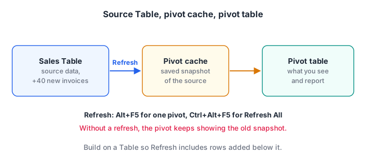
New rows reach the pivot only through Refresh. Building on a Table makes sure Refresh includes them.
- Refresh one pivot: right-click it and choose Refresh, or press Alt+F5.
- Refresh every pivot and query: Data > Refresh All, or Ctrl+Alt+F5.
- Refresh on open: PivotTable Options > Data > Refresh data when opening the file.
A VBA macro can also refresh everything as part of a weekly report job.
Quick check
You add 40 new invoices to the source Table, but the pivot total has not changed. What should you do?
A pivot reads from its pivot cache. Refresh reloads the cache, and because the source is a Table, the new rows are included.
Calculated fields and distinct counts
A calculated field adds a new measure from existing fields. Go to PivotTable Analyze > Fields, Items & Sets > Calculated Field, name it Avg Rate and enter =Amount/Qty. Excel divides the sums, so Staples shows 24100 / 85 = ₹283.53 per unit, a weighted average.
To count distinct retailers rather than invoices, tick Add this data to the Data Model when you create the pivot. Value Field Settings then offers Distinct Count, which is unavailable in a normal pivot.
Pulling a pivot value into a formula
Type = and click a pivot cell, and Excel writes a GETPIVOTDATA formula. It keeps pointing at the right value even when the pivot's layout changes:
=GETPIVOTDATA("Amount", $A$3, "Area", "Rajwada")
→ 11640
Formula-based pivots in Microsoft 365
Current Microsoft 365 builds also include GROUPBY and PIVOTBY, which return pivot-style summaries from a formula and update without refresh. =PIVOTBY(Sales[Area], Sales[Category], Sales[Amount], SUM) returns the same cross-tab as above. They are not in Excel 2016 or 2019, so classic pivot tables remain the version-safe choice.
The same pivot in pandas
pandas.pivot_table mirrors Excel's pivot. index is Rows, columns is Columns, values and aggfunc are Values, and margins=True adds grand totals.
import pandas as pd

sales = pd.DataFrame({
    "Area": ["Vijay Nagar", "Palasia", "Rajwada", "Vijay Nagar", "Bhawarkuan",
             "Palasia", "Sudama Nagar", "Rajwada", "Bhawarkuan", "Vijay Nagar"],
    "Category": ["Staples", "Staples", "Oil", "Beverages", "Staples",
                 "Staples", "Oil", "Beverages", "Staples", "Oil"],
    "Amount": [5040, 4800, 6960, 2600, 4600, 6300, 3480, 4680, 3360, 5220],
})

grid = pd.pivot_table(sales, index="Area", columns="Category", values="Amount",
                       aggfunc="sum", fill_value=0, margins=True, margins_name="Grand Total")
print(grid)

share = sales.groupby("Area")["Amount"].sum()            # Show Values As % of Grand Total
print((share / share.sum() * 100).round(1).sort_values(ascending=False))
The pandas group-by and pivot tables tutorial explains each argument. In Power BI, the same idea appears as a matrix visual, covered in dashboard design with Power BI.
Common pivot table mistakes
- Building on a fixed range. New rows below A1:I11 are ignored. Use a Table.
- Forgetting to refresh. The pivot shows old numbers and nobody notices.
- Blank or merged header cells. Excel refuses to create a pivot when a header is empty.
- Dirty categories. "Palasia" and "Palasia " become two rows. Clean first.
- Averaging averages. A calculated field divides sums; averaging per-row rates gives a different, usually wrong, figure.
Debugshala teaches Excel pivot tables in its BI Tools course built around business reporting and its Data Analytics course in Indore, both with a free demo class.
Key takeaways
- A pivot table summarises data by dragging fields into Rows, Columns, Values and Filters.
- Always build on a clean Excel Table so refresh picks up new rows.
- Value Field Settings switch Sum, Count and Average; Show Values As gives percentages and ranks.
- Group real dates into months or quarters; use a helper column for the Indian financial year.
- Slicers make pivots clickable, and Refresh (Alt+F5) is needed after every source change.
FAQ
What is a pivot table used for in Excel?
A pivot table summarises large tables quickly: totals by area, counts by product, averages by month, or percentage shares. You change the question by dragging fields instead of writing formulas. Analysts use pivots for MIS reports, reconciliations and as the base for charts and dashboards.
Why is my pivot table not updating?
Pivots read from a cached copy of the data, so they change only when you refresh. Press Alt+F5 or use Data > Refresh All. If new rows still do not appear, the source is probably a fixed range rather than an Excel Table. Change it under PivotTable Analyze > Change Data Source.
How do I show a count instead of a sum in a pivot table?
Click the field in the Values area, choose Value Field Settings, and select Count. If a number column shows Count without you choosing it, some of its values are stored as text or blank. Convert them to numbers in the source and refresh.
What is the difference between a pivot table and SUMIFS?
Both produce totals by condition. A pivot is faster to build and rearrange, so it suits exploration. SUMIFS gives a fixed layout that updates without refresh, so it suits formatted reports. Many analysts explore with a pivot, then build the final report with SUMIFS.
Are pivot tables asked in data analyst interviews in Indore?
Pivot tables are among the most common practical tasks in Excel rounds for analyst roles anywhere. Expect to build one, group dates and show percentages under time pressure. The Excel interview questions guide lists typical tasks, and Debugshala Test offers timed aptitude practice for the other rounds.
From the team behind this site
Go further with the Data Analytics Course at Debugshala
These tutorials are written by Debugshala, a training and placement institute at Old Palasia, Indore. The classroom course adds live mentoring, real projects and interview preparation.
- Offline classes at Old Palasia, Indore
- Free demo class before you pay
- Non-IT, fresher and year-gap friendly
- Placement assistance
700+ students placed · 200+ hiring partners · 4.9★ Google rating
