

Power Query in Excel: Import, Clean and Combine Data Easily
Learn Power Query in Excel step by step: import CSVs, trim and fix types, unpivot, append and merge tables, combine a folder of files and refresh in one click.
Picture the first working day of every month at a distributor in Siyaganj, Indore. The billing software exports a CSV of last month's bills. Someone opens it, deletes the top three junk rows, trims spaces from customer names, fixes dates that came in as text, looks up each product's rate, and pastes the result under last month's data.
It takes two hours, and it is never done the same way twice.
Now imagine writing that routine down once, as a recipe: "remove top 3 rows, trim Customer, change Date to a date, look up Rate from the product list".
Next month you hand Excel the new file and the recipe, and it cooks the same dish in seconds. That recipe is a query, each line is an applied step, and the kitchen where you write it is Power Query.
Power Query is Excel's built-in ETL (extract, transform, load) tool: it connects to data sources, cleans and reshapes the data through recorded steps, and loads the result into Excel, repeatable with one refresh.
If you have not cleaned data with formulas yet, read data cleaning in Excel first. Power Query does the same jobs, but in a way you never have to repeat by hand.
Where is Power Query in Excel?
In Microsoft 365, Excel 2021, 2019 and 2016 for Windows, Power Query is built in. You find it on the Data tab in the Get & Transform Data group. Excel 2010 and 2013 needed a free Microsoft add-in.
Excel for Mac in Microsoft 365 also has Power Query, though some connectors are Windows-only. Microsoft's Power Query documentation lists what each platform supports.
The same engine runs inside Power BI, so the skills transfer directly.
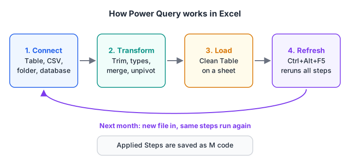
Power Query works in four stages, and the last one is what saves you hours every month.
How do you use Power Query step by step?
Start with the simplest source: a table already in your workbook. Here is a messy October export.
| Bill | Customer | SKU | Qty |
|---|---|---|---|
| 501 | Gupta Kirana |
AT10 | 5 |
| 502 | Jain Stores |
TD01 | 12 |
| 503 | Gupta Kirana |
SO01 | 8 |
A pivot table would treat " Gupta Kirana" and "Gupta Kirana" as two customers.
- Click inside the data, press Ctrl+T to make it a Table, and name it
OctSales. - Choose Data > From Table/Range. The Power Query Editor opens in a new window.
- Select the Customer column, then Transform > Format > Trim. A step called "Trimmed Text" appears in the Applied Steps pane on the right.
- Select the Qty column and set its type to Whole Number with the type icon in the column header.
- Choose Home > Close & Load. Excel writes the cleaned data to a new sheet as a Table.
Click any step in Applied Steps to see the data at that point. That is how you debug a query.
Loading from a CSV file instead
For a file on disk, use Data > Get Data > From File > From Text/CSV and click Transform Data instead of Load. You land in the same editor.
Which Power Query transformations do you use most?
Most monthly cleaning needs a handful of ribbon commands.
| Task | Where in the editor | Formula equivalent |
|---|---|---|
| Remove junk top rows | Home > Remove Rows > Remove Top Rows | Deleting rows by hand |
| Use first row as headers | Home > Use First Row as Headers | — |
| Trim spaces | Transform > Format > Trim | TRIM() |
| Split "Indore-MP" into two columns | Home > Split Column > By Delimiter | TEXTBEFORE(), TEXTAFTER() |
| Fill blanks with the value above | Transform > Fill > Down | Go To Special + formula |
| Remove duplicates | Right-click column > Remove Duplicates | Data > Remove Duplicates |
| Filter out blank or zero rows | Filter arrow on the column header | FILTER() |
| Wide months to long rows | Transform > Unpivot Other Columns | No simple equivalent |
| Totals by group | Home > Group By | Pivot table or SUMIFS() |
The formula column links back to Excel text and date functions. Formulas must be copied down; Power Query steps apply to every row automatically.
Fixing Indian dates (dd-mm-yyyy)
Billing software in India usually writes dates as 05-11-2026 for 5 November. If your Windows region is set to the US, Power Query may read that as 11 May, or fail. Right-click the Date column and choose Change Type > Using Locale, then pick Date and English (India). The step uses the "en-IN" culture, so the day comes first.
Unpivot: turn a wide report into a proper table
Many reports arrive "wide", with one column per month, which is hard to filter or pivot.
| Product | Aug | Sep | Oct |
|---|---|---|---|
| Atta 10kg | 41,000 | 45,500 | 52,300 |
| Toor Dal 1kg | 15,200 | 14,800 | 16,900 |
Select the Product column and choose Transform > Unpivot Other Columns. You get one row per product per month, with columns Product, Attribute and Value, which you rename to Month and Sales. Six tidy rows replace two wide ones, and a new month column next year is unpivoted automatically.
What is M code in Power Query?
Every button you click writes a line of a language called M (the Power Query formula language). Open Home > Advanced Editor to see it. A query is a let block of named steps, and in names the step to return.
let
    Source  = Excel.CurrentWorkbook(){[Name="OctSales"]}[Content],
    Trimmed = Table.TransformColumns(Source, {{"Customer", Text.Trim, type text}}),
    Typed   = Table.TransformColumnTypes(Trimmed, {{"Bill", Int64.Type}, {"Qty", Int64.Type}}),
    NoZero  = Table.SelectRows(Typed, each [Qty] > 0)
in
    NoZero
Each step takes the previous step's name as its input. You rarely write M from scratch, but reading it helps you fix a broken source path. The Power Query M reference documents every function.
How do you combine data with Append and Merge?
There are two ways to combine tables, and mixing them up is the most common beginner mistake.
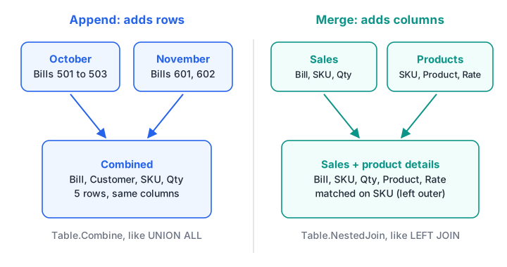
Append adds rows. Merge adds columns.
| Append | Merge | |
|---|---|---|
| What it does | Stacks tables on top of each other | Joins two tables side by side on a key |
| Needs | Same column names | A shared key column, such as SKU |
| Result | More rows | More columns |
| SQL equivalent | UNION ALL |
LEFT JOIN (or other join kinds) |
| M function | Table.Combine |
Table.NestedJoin |
To append, open the October query and choose Home > Append Queries, then pick the November query. To merge, choose Home > Merge Queries, select the SKU column in both tables, choose Left Outer as the join kind, then click the expand icon on the new column and tick Product and Rate.
Think of Merge as XLOOKUP for an entire table at once.
Combine every file in a folder
The real time-saver is Data > Get Data > From File > From Folder. Point it at a folder of monthly CSVs and click Combine & Transform Data. Excel builds helper queries and stacks all the files. Drop December's file into the folder, press Refresh, and it joins the rest.
Quick check
You have separate tables for April, May and June sales with identical columns. Which Power Query command combines them into one table?
Append stacks tables with the same columns on top of each other. Merge joins tables side by side on a key column.
The same append, merge and group in pandas
Power Query and pandas solve the same problems:
import pandas as pd

# Two monthly exports from billing software (note the messy spaces)
oct_sales = pd.DataFrame({"Bill": [501, 502, 503],
                          "Customer": [" Gupta Kirana", "Jain Stores ", "Gupta Kirana"],
                          "SKU": ["AT10", "TD01", "SO01"], "Qty": [5, 12, 8]})
nov_sales = pd.DataFrame({"Bill": [601, 602],
                          "Customer": ["Mehta General", " Jain Stores"],
                          "SKU": ["AT10", "SG05"], "Qty": [7, 10]})
products = pd.DataFrame({"SKU": ["AT10", "TD01", "SO01", "SG05"],
                         "Product": ["Atta 10kg", "Toor Dal 1kg", "Sunflower Oil 1L", "Sugar 5kg"],
                         "Rate": [460, 160, 175, 240]})

# Append (Table.Combine): stack rows with the same columns
sales = pd.concat([oct_sales, nov_sales], ignore_index=True)
# Trim (Text.Trim)
sales["Customer"] = sales["Customer"].str.strip()
# Merge (Table.NestedJoin, left outer): bring in product name and rate
sales = sales.merge(products, on="SKU", how="left")
sales["Amount"] = sales["Qty"] * sales["Rate"]
print(sales[["Bill", "Customer", "Product", "Qty", "Amount"]])

# Group By (Table.Group): total per customer
print(sales.groupby("Customer")["Amount"].sum().sort_values(ascending=False))
After trimming, Jain Stores is one customer with ₹4,320 instead of two half-customers. The unpivot step is melt in pandas:
import pandas as pd

# A "wide" report: one column per month, which is hard to filter or pivot
wide = pd.DataFrame({"Product": ["Atta 10kg", "Toor Dal 1kg"],
                     "Aug": [41000, 15200], "Sep": [45500, 14800], "Oct": [52300, 16900]})
print(wide)

# Unpivot Other Columns = melt: one row per product per month
long = wide.melt(id_vars="Product", var_name="Month", value_name="Sales")
print(long)
For a deeper look at the pandas side, see data cleaning with pandas.
How do you refresh a Power Query?
Press Ctrl+Alt+F5 or choose Data > Refresh All to rerun every query. To refresh one query, right-click its output table and choose Refresh.
For hands-off updates, open Data > Queries & Connections, right-click the query, choose Properties, and tick Refresh data when opening the file or Refresh every n minutes.
Common Power Query mistakes
- Editing the output table by hand. The next refresh overwrites it. Make changes as steps in the query instead.
- Hard-coded file paths. If the source file moves, the Source step breaks. Fix it in Home > Data Source Settings.
- Changing types too early. The automatic "Changed Type" step locks column names; if a column is renamed in the source, it errors. Delete that step and set types after cleaning.
- Merging on dirty keys. "AT10 " will not match "AT10". Trim keys first.
Once your data loads clean, you can build charts on it, as in Excel charts and dashboards, or automate what is left with macros in the Excel macros tutorial. Debugshala's Data Analytics course includes Excel, so if you want these data-prep habits drilled in class, an analytics course in Indore built around real data preparation is worth a demo class.
Quick check
Why should you not type corrections directly into a table loaded by Power Query?
A refresh rebuilds the output from the source and steps. Put corrections into the query as steps so they run every time.
Key takeaways
- Power Query lives on the Data tab (Get & Transform) in Excel 2016 and later, including Microsoft 365.
- Every action is saved as an applied step, written in the M language.
- Append adds rows from tables with the same columns; Merge adds columns by matching a key.
- Use Change Type > Using Locale with English (India) for dd-mm-yyyy dates.
- Refresh with Ctrl+Alt+F5, and never hand-edit a query's output.
FAQ
What is Power Query used for in Excel?
Power Query is used to import data from files, folders, databases and the web, clean it with repeatable steps, and load it into Excel. Typical jobs are trimming spaces, fixing types, removing junk rows, combining monthly files and joining a sales list to a product master. You set it up once and refresh it every month.
Is Power Query better than VLOOKUP?
For joining whole tables, usually yes. A Power Query merge matches every row in one step, does not slow the workbook with thousands of formulas, and survives new data with a refresh. For a single quick lookup inside a report, XLOOKUP or VLOOKUP is still simpler and more transparent to the reader.
Do I need to learn M code to use Power Query?
No. Almost everything is done with ribbon buttons, and Power Query writes the M code for you. Learning to read M helps when you need to rename steps, change a file path, or add a custom column with a condition. Most analysts edit small pieces of M rather than writing it from scratch.
What is the difference between Power Query and Power Pivot?
Power Query gets and cleans data. Power Pivot models it: it stores large tables in the Data Model, creates relationships between them, and adds DAX measures for pivot tables. In practice you use Power Query first to prepare tables, then Power Pivot to analyse them. Power BI combines both.
Where can I learn Excel for data analysis in Indore?
Debugshala teaches Excel as part of its Data Analytics and BI Tools courses at Old Palasia, Indore. The courses are open to non-IT graduates, include placement assistance and start with a free demo class. Test what you know with free quizzes at Debugshala Test.
From the team behind this site
Go further with the Data Analytics Course at Debugshala
These tutorials are written by Debugshala, a training and placement institute at Old Palasia, Indore. The classroom course adds live mentoring, real projects and interview preparation.
- Offline classes at Old Palasia, Indore
- Free demo class before you pay
- Non-IT, fresher and year-gap friendly
- Placement assistance
700+ students placed · 200+ hiring partners · 4.9★ Google rating
