

XLOOKUP vs VLOOKUP vs INDEX MATCH in Excel, with Examples
XLOOKUP vs VLOOKUP vs INDEX MATCH: syntax, exact and approximate match, left lookups, last match, two-criteria lookups and which one to use in which version.
The billing clerk at Narmada Traders types only a product code, such as P103, on each order line. Before the invoice prints, someone has to find that code in the product price list and copy the product name, category and rate beside it. With 300 order lines a day, doing it by eye means mistakes.
The price list is a reference table. The order sheet is where you need its values. Matching one to the other, row by row, is a lookup.
The product code is the lookup value. The Code column of the price list is the lookup array, and the Rate column is the return array. Hand those three to a function and Excel fetches the rate for every row.
XLOOKUP is an Excel lookup function that searches one range for a value and returns the matching item from another range, replacing the older VLOOKUP, HLOOKUP and most INDEX MATCH formulas.
Here is the product master, saved as an Excel Table named Products.
| Code | Product | Category | Rate | Stock |
|---|---|---|---|---|
| P101 | Atta 10kg | Staples | 420 | 140 |
| P102 | Toor Dal 1kg | Staples | 160 | 300 |
| P103 | Sunflower Oil 1L | Oil | 145 | 520 |
| P104 | Tea 500g | Beverages | 260 | 90 |
| P105 | Sugar 5kg | Staples | 230 | 210 |
What is VLOOKUP and how does it work?
VLOOKUP (vertical lookup) searches the first column of a range and returns a value from a column you specify by number, counting from the left.
=VLOOKUP(lookup_value, table_array, col_index_num, [range_lookup])
=VLOOKUP("P103", Products, 4, FALSE)
→ 145
Read it as: "find P103 in the first column of Products, then go across to column 4 and return that." Rate is the fourth column, so the answer is 145.
The last argument decides the match type. FALSE (or 0) means exact match. If you leave it out, VLOOKUP assumes TRUE, an approximate match, which on an unsorted list can return a wrong rate with no error at all.
Where VLOOKUP breaks
- It cannot look left. To find the code for "Tea 500g", the search column (Product) is to the right of the answer (Code). VLOOKUP cannot do it.
- Column numbers are fragile. Insert an MRP column before Rate and
4now points at MRP. Every VLOOKUP silently returns the wrong figure. - It returns only the first match. For the latest order from a retailer, you need another approach.
Quick check
On a price list that is not sorted by Code, =VLOOKUP("P104", Products, 4) returns a wrong rate. What is the most likely fix?
Without the fourth argument, VLOOKUP uses approximate match, which needs the first column sorted. Adding FALSE forces an exact match on the code.
How does INDEX MATCH work?
MATCH finds the position of a value in a single column. INDEX returns the item at a given position. Together they look up in any direction.
=MATCH("Tea 500g", Products[Product], 0)                       → 4
=INDEX(Products[Code], MATCH("Tea 500g", Products[Product], 0)) → P104
The 0 in MATCH means exact match. Because you name the return column directly, inserting columns does not break it.
INDEX MATCH works in every Excel version still in use, so it is the formula to use when a workbook must open on an older office laptop. It also supports a two-way lookup: =INDEX(grid, MATCH(row_label, row_headers, 0), MATCH(col_label, col_headers, 0)).
How does XLOOKUP work?
XLOOKUP takes the lookup range and the return range separately, so there is no column counting and no direction limit.
=XLOOKUP(lookup_value, lookup_array, return_array, [if_not_found], [match_mode], [search_mode])
=XLOOKUP("P103", Products[Code], Products[Rate])
→ 145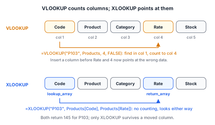
VLOOKUP depends on a column number. XLOOKUP points at the return column directly, so moving columns cannot break it.
Microsoft's XLOOKUP reference lists the defaults: exact match (match_mode 0) and search from first to last (search_mode 1). XLOOKUP is available in Microsoft 365, Excel 2021, Excel 2024 and Excel for the web, but not in Excel 2016 or 2019.
Handle "not found" without IFERROR
The fourth argument is what to show when nothing matches.
=XLOOKUP("P109", Products[Code], Products[Rate], "Code not in master")
→ Code not in master
Look to the left
The same function finds a code from a product name, with no rearranging.
=XLOOKUP("Tea 500g", Products[Product], Products[Code])
→ P104
Return several columns at once
Give a return range that spans several adjacent columns, and the answer spills across.
=XLOOKUP("P103", Products[Code], Products[[Category]:[Rate]])
→ Oil | 145
Find the last match
Set search_mode to -1 to search from the bottom up. On the Sales Table from the IF function tutorial, this returns Sharma Kirana's latest invoice.
=XLOOKUP("Sharma Kirana", Sales[Retailer], Sales[Invoice], , 0, -1)
→ NT-1010
Look up with two conditions
Multiply two TRUE/FALSE tests and look for the 1. Patel Provision's tea order:
=XLOOKUP(1, (Sales[Retailer]="Patel Provision")*(Sales[Product]="Tea 500g"), Sales[Invoice])
→ NT-1008
Quick check
Which XLOOKUP returns the most recent invoice for Gupta Mart from the Sales Table?
search_mode -1 searches from the last row upwards, so it returns NT-1009 rather than the first match, NT-1005.
Approximate match: slabs and rate bands
Not every lookup wants an exact match. The discount slabs from the last tutorial can live in a small Table named Slabs, sorted from smallest to largest.
| From (₹) | Discount |
|---|---|
| 0 | 0% |
| 4000 | 3% |
| 6000 | 5% |
match_mode -1 means "exact, or else the next smaller item". A ₹5,040 bill has no exact row, so XLOOKUP falls back to 4000 and returns 3%.
=XLOOKUP([@Amount], Slabs[From], Slabs[Discount], , -1)
→ 3% for 5040, 5% for 6960, 0% for 2600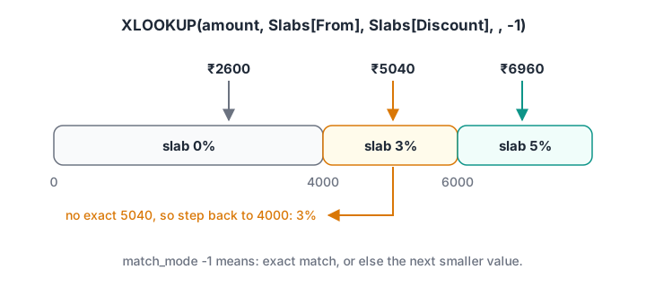
With match_mode -1, XLOOKUP steps back to the largest slab that is not above the amount.
The VLOOKUP version is =VLOOKUP([@Amount], Slabs, 2, TRUE). It gives the same answer but only if the From column is sorted ascending. XLOOKUP with -1 does not need sorting. Change a slab in the table and every invoice updates, which is far easier than editing a nested IF.
XLOOKUP vs VLOOKUP vs INDEX MATCH compared
| Feature | VLOOKUP | INDEX MATCH | XLOOKUP |
|---|---|---|---|
| Default match | Approximate (must add FALSE) | Depends on MATCH's third argument | Exact |
| Look left | No | Yes | Yes |
| Survives inserted columns | No | Yes | Yes |
| Built-in "not found" text | No (wrap in IFNA) | No (wrap in IFNA) | Yes |
| Last match | No | Not easily | Yes (search_mode -1) |
| Return several columns | One per formula | One per formula | Yes, spills |
| Works in Excel 2016/2019 | Yes | Yes | No |
Which should you use? XLOOKUP for any new work in Microsoft 365. INDEX MATCH when the file must work in older versions. Learn to read VLOOKUP, because older office workbooks are full of it and interviewers still ask about it.
The same lookup in pandas
A column of lookups is a left join in pandas. merge with how="left" keeps every order line and fills unmatched ones with NaN, which you can replace like XLOOKUP's if_not_found. merge_asof performs the approximate-match slab lookup.
import pandas as pd

products = pd.DataFrame({"Code": ["P101", "P102", "P103", "P104", "P105"],
                         "Product": ["Atta 10kg", "Toor Dal 1kg", "Sunflower Oil 1L",
                                     "Tea 500g", "Sugar 5kg"],
                         "Rate": [420, 160, 145, 260, 230]})
orders = pd.DataFrame({"Line": [1, 2, 3, 4], "Code": ["P103", "P101", "P109", "P104"],
                       "Qty": [48, 12, 5, 10]})

# Like =XLOOKUP([@Code], Products[Code], Products[Rate], "Code not in master")
lines = orders.merge(products, on="Code", how="left")
lines["Product"] = lines["Product"].fillna("Code not in master")
lines["Amount"] = lines["Qty"] * lines["Rate"]
print(lines.to_string(index=False))

# Like =XLOOKUP(amount, Slabs[From], Slabs[Discount], , -1)
slabs = pd.DataFrame({"From": [0, 4000, 6000], "Discount": [0.0, 0.03, 0.05]})
bills = pd.DataFrame({"Amount": [2600, 5040, 6960]})
print(pd.merge_asof(bills, slabs, left_on="Amount", right_on="From").to_string(index=False))
The SQL equivalent is a LEFT JOIN, covered in the SQL joins tutorial.
Common lookup mistakes
- Leaving out FALSE in VLOOKUP. You get approximate matching and plausible but wrong numbers.
- Trailing spaces in keys. "P103 " never matches "P103". Clean keys with TRIM, as shown in the text and date functions tutorial.
- Numbers vs text. A code typed as the number 1001 does not match the text "1001". Make both sides the same type.
- Duplicate keys in the master. Every lookup returns only the first match, so a duplicated code hides the second row. Check with
=COUNTIFS(Products[Code], [@Code])>1. - Hard-coded ranges such as A2:E6. New products fall outside them. Use Table references.
Key takeaways
- A lookup fetches a related value from a reference table using a shared key.
- XLOOKUP defaults to exact match, looks in any direction, and has built-in not-found text.
- VLOOKUP needs FALSE for exact match and breaks when columns move.
- INDEX MATCH is the version-safe alternative for Excel 2016 and 2019.
- Approximate match (
match_mode-1) turns a small slab table into a flexible rule.
FAQ
Is XLOOKUP better than VLOOKUP?
Yes, for almost every task. XLOOKUP defaults to exact match, can look left, survives inserted columns, returns several columns and finds the last match. The only reason to keep VLOOKUP or INDEX MATCH is compatibility with Excel 2016 or 2019, where XLOOKUP shows #NAME?.
Why is my XLOOKUP returning #N/A?
#N/A means no match was found. Common causes are extra spaces, a number stored as text on one side, or a spelling difference. Check with =LEN() on both values, clean with TRIM, or add the if_not_found argument so missing keys show a clear message instead.
Can XLOOKUP return multiple values?
Yes. If the return array covers several columns, the result spills across those columns. To return every matching row rather than the first, use FILTER instead: =FILTER(Sales[Invoice], Sales[Retailer]="Sharma Kirana") lists all three Sharma Kirana invoices.
Do interviewers still ask about VLOOKUP?
Yes. Many analyst interviews ask you to explain VLOOKUP's limits and then solve the same task with XLOOKUP or INDEX MATCH. The Excel interview questions guide covers typical lookup tasks, and aptitude rounds can be practised on Debugshala Test.
Is there a classroom data analytics course in Indore for beginners?
Yes. Debugshala, an IT training and placement institute at Old Palasia, teaches Excel lookups as part of its classroom Data Analytics training with placement assistance. Classes are taught in English and Hindi, beginners from non-IT backgrounds are accepted, and a free demo class lets you see the teaching style first.
From the team behind this site
Go further with the Data Analytics Course at Debugshala
These tutorials are written by Debugshala, a training and placement institute at Old Palasia, Indore. The classroom course adds live mentoring, real projects and interview preparation.
- Offline classes at Old Palasia, Indore
- Free demo class before you pay
- Non-IT, fresher and year-gap friendly
- Placement assistance
700+ students placed · 200+ hiring partners · 4.9★ Google rating
