

Excel Charts and Dashboard Tutorial: Build a Sales Dashboard
Learn which Excel chart to use, then build a sales dashboard with KPI cells, SUMIFS, pivot charts, slicers and sparklines that updates when data changes.
Imagine you are the accounts person at Narmada Traders, a grocery distributor in Indore that supplies kirana stores in Vijay Nagar, Palasia and Rajwada. Every Monday the owner asks the same three questions: how much did we sell, which area is growing, and which product is carrying us?
You could send him a sheet with 2,000 rows. He will scroll for ten seconds and call you anyway. Or you could send one screen with three numbers at the top and two charts below, where the answers jump out before he finishes his chai.
That one screen is a dashboard. The 2,000 rows are your data table, the three numbers are KPIs (key performance indicators), and the charts are the visuals that turn columns of rupees into a shape the eye can read.
An Excel dashboard is a single worksheet that summarises a dataset with a few KPI cells, charts and filters, all linked to the data so it refreshes automatically.
If you are new to Excel, start with Excel for data analysis and come back once you are comfortable with tables and formulas.
Which Excel chart should you use?
A chart answers one question. Write the question in plain words first, then pick the chart that answers it fastest.
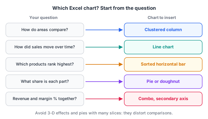
Start from the question, not from the chart gallery.
| Your question | Best chart | Avoid |
|---|---|---|
| How do areas or months compare? | Clustered column | 3-D column |
| How did sales move over 12 months? | Line | Pie, area with many series |
| Which products rank highest? | Bar (horizontal), sorted | Unsorted column |
| What share does each part have? | Pie or doughnut, 2 to 4 slices | Pie with 9 slices |
| Revenue and margin % together? | Combo with secondary axis | Two separate charts |
| How is order value spread out? | Histogram (Excel 2016+) | Line |
Use a horizontal bar chart for product names, because long labels like "Sunflower Oil 1L" fit without tilting. Sort it largest first.
Waterfall, Histogram, Pareto, Treemap and Sunburst charts need Excel 2016 or later; Funnel and Filled Map charts came later: Microsoft's current help lists Funnel for Excel 2021 and later or a Microsoft 365 subscription, so check before you rely on either in an older office copy.
Quick check
You want to show how monthly revenue changed over 12 months. Which chart fits best?
A line chart shows movement over time most clearly. Pies show parts of a whole, and 3-D effects distort values.
How do you create a chart in Excel?
Charts behave best when their source is an Excel Table, because the chart grows when you add rows. Here is the sample data for this tutorial.
| Date | Area | Product | Amount (₹) |
|---|---|---|---|
| 04-07-2026 | Vijay Nagar | Atta 10kg | 18,400 |
| 11-07-2026 | Palasia | Toor Dal 1kg | 9,600 |
| 19-07-2026 | Rajwada | Sugar 5kg | 7,200 |
| 26-07-2026 | Vijay Nagar | Sunflower Oil 1L | 12,600 |
| … 8 more rows to 27-09-2026 |
Follow these steps to make your first chart:
- Click any cell in the data and press Ctrl+T to turn it into a Table. Name it
Salesin Table Design > Table Name. - Build a small summary next to it (the next section shows the formulas). Charts read better from a summary than from raw rows.
- Select the summary and choose Insert > Recommended Charts. Excel suggests charts that fit the shape of your data.
- Pick Clustered Column and click OK. Press Alt+F1 instead if you want the default chart in one keystroke, or F11 to put it on its own chart sheet.
- Click the + button beside the chart to switch chart elements on or off: axis titles, data labels, legend.
- Give the chart a title that states the finding, such as "Rajwada overtook Palasia in September", not just "Sales".
Format charts so they read in two seconds
Delete what carries no information: gridlines once you add data labels, the legend for a single series, and every 3-D effect, which distorts heights.
Use one strong colour for the bar you want the reader to notice and grey for the rest. Format numbers in the axis as ₹#,##0 or in thousands (₹#,##0,"K") so the axis does not shout seven-digit figures.
How do you build a simple sales dashboard in Excel?
A dashboard that survives next month has three layers. Keep them on separate sheets: Data, Calc and Dashboard.
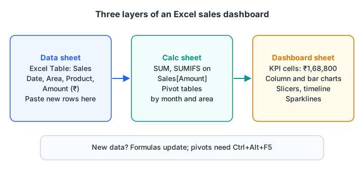
Data flows one way: raw table, then calculations, then the screen the owner sees.
Step 1: KPI cells with formulas
On the Calc sheet, compute the headline numbers from the Sales table using structured references. These keep working when the table grows.
Total revenue        =SUM(Sales[Amount])                     → 168800
Orders               =ROWS(Sales[Amount])                    → 12
Average order value  =ROUND(AVERAGE(Sales[Amount]), 0)       → 14067
Vijay Nagar, Sep     =SUMIFS(Sales[Amount], Sales[Area], "Vijay Nagar",
                        Sales[Date], ">="&DATE(2026,9,1),
                        Sales[Date], "<"&DATE(2026,10,1))     → 10200
The SUMIFS pattern is explained in detail in Excel formulas and functions. On the dashboard sheet, link big cells to these results (=Calc!B2) and format them with a large font.
Step 2: the area-by-month summary
You can build the chart's source with a pivot table (Insert > PivotTable, Month in Rows, Area in Columns, Amount in Values) or with formulas. Here is what the summary should return.
| Month | Palasia | Rajwada | Vijay Nagar |
|---|---|---|---|
| Jul 2026 | 9,600 | 7,200 | 31,000 |
| Aug 2026 | 27,900 | 8,800 | 19,900 |
| Sep 2026 | 23,800 | 30,400 | 10,200 |
If you use a pivot table, insert the chart with PivotTable Analyze > PivotChart. A PivotChart follows the pivot's filters, which is what makes slicers possible. The full pivot workflow is in Excel pivot tables.
Step 3: slicers, timelines and sparklines
Slicers are clickable filter buttons. Select a pivot table, choose PivotTable Analyze > Insert Slicer and tick Area. To make one slicer filter every chart, right-click it, choose Report Connections and tick each pivot table.
A timeline is a slicer for dates (PivotTable Analyze > Insert Timeline). It lets the owner drag across months instead of ticking boxes.
Sparklines are tiny charts inside one cell. Select an empty cell beside each area's row and choose Insert > Sparklines > Line. They show a trend without taking a full chart's space.
Step 4: lay out the screen
Put KPI cells across the top, the most important chart top-left (where the eye lands first), and slicers on the side. Line the charts up on the grid by holding Alt while you drag, which snaps them to cell edges.
Hide gridlines with View > Gridlines.
How do you make an Excel dashboard update automatically?
With three layers you only ever touch the Data sheet. Paste new rows under the Sales table and the formulas pick them up at once.
Pivot tables are different: they cache their data. Press Ctrl+Alt+F5 (Data > Refresh All) after you add data, or the pivot charts will show last week's numbers.
If your data arrives as a CSV export from billing software, load it through Power Query so a refresh pulls the new file and cleans it the same way each time. That is the next article: Power Query in Excel.
Quick check
You added 50 new rows to the Sales table, but the PivotChart has not changed. What should you do?
Pivot tables keep a cache of the data. Refresh All (Ctrl+Alt+F5) updates the cache; F9 only recalculates formulas.
The same dashboard numbers in pandas
If you know Python, this pandas version computes the same KPI and chart data, a handy check on your Excel numbers.
import pandas as pd

sales = pd.DataFrame({
    "Date": pd.to_datetime(["2026-07-04", "2026-07-11", "2026-07-19", "2026-07-26",
                            "2026-08-02", "2026-08-09", "2026-08-17", "2026-08-24",
                            "2026-09-03", "2026-09-12", "2026-09-20", "2026-09-27"]),
    "Area": ["Vijay Nagar", "Palasia", "Rajwada", "Vijay Nagar",
             "Palasia", "Rajwada", "Vijay Nagar", "Palasia",
             "Rajwada", "Vijay Nagar", "Palasia", "Rajwada"],
    "Product": ["Atta 10kg", "Toor Dal 1kg", "Sugar 5kg", "Sunflower Oil 1L",
                "Atta 10kg", "Toor Dal 1kg", "Atta 10kg", "Sugar 5kg",
                "Sunflower Oil 1L", "Toor Dal 1kg", "Atta 10kg", "Atta 10kg"],
    "Amount": [18400, 9600, 7200, 12600, 21500, 8800, 19900, 6400,
               14100, 10200, 23800, 16300],
})

# KPI cells: what the top row of the dashboard shows
print("Total revenue:", sales["Amount"].sum())
print("Orders:", len(sales))
print("Average order value:", round(sales["Amount"].mean()))

# Data behind the column chart: month by area, like a pivot table
sales["Month"] = sales["Date"].dt.strftime("%Y-%m")
pivot = sales.pivot_table(index="Month", columns="Area", values="Amount",
                          aggfunc="sum", fill_value=0)
print(pivot)

# Data behind the bar chart: product ranking
print(sales.groupby("Product")["Amount"].sum().sort_values(ascending=False))
Atta 10kg brings in ₹99,900 of the ₹1,68,800 total, so it belongs at the top of the bar chart. More on this style of summary is in pandas groupby and pivot tables.
Common Excel dashboard mistakes
- Charting raw rows. A chart of 2,000 transactions is noise. Summarise first, then chart the summary.
- Typed numbers in KPI cells. If someone overwrites a formula with a typed figure, the dashboard silently stops updating. Protect the dashboard sheet (Review > Protect Sheet) once it is done.
- Too many charts. Five to seven visuals is plenty. If the owner needs more, it is a second dashboard.
- Forgetting to refresh pivots. Formulas update instantly; pivot tables do not.
- Rainbow colours. Colour should mean something, such as highlighting the area that missed target.
When your dashboards outgrow one workbook or need to be shared online with many users, a BI tool is the next step. Dashboard design in Power BI covers the same principles at a larger scale. Debugshala teaches Excel dashboards like this one, and the step up to BI reports, in its BI Tools course in Indore.
Key takeaways
- Start every chart from a written question, then choose the chart type that answers it.
- Keep three layers: a data Table, a calculation sheet, and the dashboard sheet.
- Use structured references such as
Sales[Amount]so formulas grow with the data. - Slicers, timelines and sparklines add interactivity without any code.
- Refresh pivot tables after new data arrives; formulas update on their own.
FAQ
How do I make a dashboard in Excel for beginners?
Make your data an Excel Table with Ctrl+T, build a summary with SUMIFS formulas or a pivot table, then insert charts from that summary onto a separate sheet. Add KPI cells linked to the summary and a slicer for filtering. That three-sheet layout is enough for most small business dashboards.
What is the difference between a chart and a PivotChart in Excel?
A normal chart reads a fixed cell range or table. A PivotChart is tied to a pivot table, so it follows the pivot's fields and filters, and slicers can control it. Use a PivotChart when you want the reader to filter by area, product or month with a click.
Can Excel dashboards update automatically?
Yes, if every number comes from formulas that point at an Excel Table. Formulas update as soon as you add rows. Pivot tables and Power Query need a refresh, which you trigger with Data > Refresh All or set to run when the file opens in the connection properties.
Do Excel 2016 and 2019 support slicers and sparklines?
Yes. Sparklines arrived in Excel 2010, slicers for pivot tables in 2010, and timelines in 2013, so Excel 2016 and 2019 have all three. What they lack are dynamic array functions such as FILTER and UNIQUE, and Excel 2016 also lacks newer chart types like Funnel and Filled Map.
Where can I learn Excel dashboards in Indore?
Debugshala teaches Excel, from charts and pivot tables to macros, in its Data Analytics and BI Tools courses at the Old Palasia campus in Indore. Classes run in English and Hindi, and you can attend a free demo class before you pay. You can also test yourself with free quizzes on Debugshala Test.
From the team behind this site
Go further with the Data Analytics Course at Debugshala
These tutorials are written by Debugshala, a training and placement institute at Old Palasia, Indore. The classroom course adds live mentoring, real projects and interview preparation.
- Offline classes at Old Palasia, Indore
- Free demo class before you pay
- Non-IT, fresher and year-gap friendly
- Placement assistance
700+ students placed · 200+ hiring partners · 4.9★ Google rating
